Tutorial about fluopy - two Cy5 in dSTORM simulation

Here we outline a simulation procedure for a 2-fluorophore Cy5 system under dSTORM conditions.

from pprint import pprint

%matplotlib inline

import matplotlib.pyplot as plt
import numpy as np

import fluopy
import fluopy.analysis as an
import fluopy.blinking as bl
import fluopy.emissions as em
import fluopy.fcs as fcs_p
import fluopy.figure as fi
import fluopy.fluorophores as fl
import fluopy.formulas as fo
import fluopy.miscellaneous as mi
import fluopy.prediction as pr
import fluopy.simulation as si
import fluopy.transitions as tr

fluopy.__version__

'0.2.0'

rng = np.random.default_rng(seed=1)

Define the fluorophore system

fluorophores = fl.construct_fluorophores(
    name="cy5_dna", distance=10, count=2, shape=None
)
fluorophore_system = fl.FluorophoreSystem(fluorophores=fluorophores)

pprint(vars(fluorophore_system))

{'count': 2,
 'distances': {(0, 1): np.float64(10.0), (1, 0): np.float64(10.0)},
 'fluorophores': [Fluorophore(identity=0,
                              name='cy5_dna',
                              position=array([0, 0]),
                              constants=FluorophoreData(data_files='cy5_data',
                                                        QUANTUM_YIELD=0.27,
                                                        FLUORESCENCE_LIFETIME=1.7e-09,
                                                        S1_QUENCH_RATE=0,
                                                        ISC_ST_RATE=830000.0,
                                                        ISC_TS_RATE=5000.0,
                                                        RISC_RATE=0,
                                                        STA_EFFICIENCY=0,
                                                        PHOTOBLEACH_T1_RATE=10.0,
                                                        PHOTOBLEACH_T2_RATE=0,
                                                        DSTORM_PET_T_RATE_MOL=100000000.0,
                                                        DSTORM_PET_S_RATE_MOL=1000000000.0,
                                                        DSTORM_PET_SUCCESS_RATE=0.001,
                                                        DSTORM_TH_EL_RATE_1=0.01,
                                                        DSTORM_TH_EL_RATE_2=0,
                                                        DSTORM_P_EL_CROSS_SECTION=6e-24,
                                                        RAD_ESCAPE_EFFICIENCY=0.01,
                                                        RAD_RELAX_RATE=1300.0,
                                                        OFRET_EFFICIENCY=0.001,
                                                        ISO_RATE=4000000.0,
                                                        BISO_CROSS_SECTION=6e-18,
                                                        BISO_THERMAL_RATE=5000.0,
                                                        BISO_EFFICIENCY=0.04,
                                                        H2O_ATTACK_S=0,
                                                        H2O_ATTACK_T=0,
                                                        BACK_REACTION=0)),
                  Fluorophore(identity=1,
                              name='cy5_dna',
                              position=array([10,  0]),
                              constants=FluorophoreData(data_files='cy5_data',
                                                        QUANTUM_YIELD=0.27,
                                                        FLUORESCENCE_LIFETIME=1.7e-09,
                                                        S1_QUENCH_RATE=0,
                                                        ISC_ST_RATE=830000.0,
                                                        ISC_TS_RATE=5000.0,
                                                        RISC_RATE=0,
                                                        STA_EFFICIENCY=0,
                                                        PHOTOBLEACH_T1_RATE=10.0,
                                                        PHOTOBLEACH_T2_RATE=0,
                                                        DSTORM_PET_T_RATE_MOL=100000000.0,
                                                        DSTORM_PET_S_RATE_MOL=1000000000.0,
                                                        DSTORM_PET_SUCCESS_RATE=0.001,
                                                        DSTORM_TH_EL_RATE_1=0.01,
                                                        DSTORM_TH_EL_RATE_2=0,
                                                        DSTORM_P_EL_CROSS_SECTION=6e-24,
                                                        RAD_ESCAPE_EFFICIENCY=0.01,
                                                        RAD_RELAX_RATE=1300.0,
                                                        OFRET_EFFICIENCY=0.001,
                                                        ISO_RATE=4000000.0,
                                                        BISO_CROSS_SECTION=6e-18,
                                                        BISO_THERMAL_RATE=5000.0,
                                                        BISO_EFFICIENCY=0.04,
                                                        H2O_ATTACK_S=0,
                                                        H2O_ATTACK_T=0,
                                                        BACK_REACTION=0))],
 'multi_type': False}

Define the transition set

transitions = fluorophore_system.load_transitions(
    summarize=True,
    irradiance=2,
    wavelength=640,
    bleaching=False,
    energy_transfer=True,
    dstorm=True,
)
transition_set = tr.TransitionSet(transitions, fluorophore_system)
transition_set.finalize()

<fluopy.transitions.TransitionSet at 0x7009103def90>

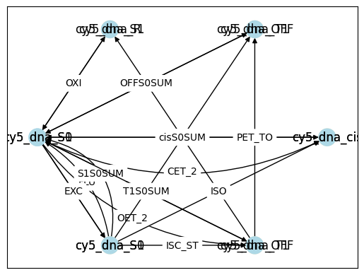
transition_set.plot(graph_type="shell", colors=None, scale=1);

transition_set.transition_df

		transition_type	abbreviation	initial_state	final_state	rate	photon	fluorophore_ids	absorbing
Fluorophore	identity
cy5_dna	0	TransitionType.EXCITATION	EXC	SingleState.S0	SingleState.S1	5.815700e+06	False	[0, 1]	False
	1	TransitionType.FLUORESCENT_EMISSION	FLU	SingleState.S1	SingleState.S0	1.588235e+08	True	[0, 1]	False
	2	TransitionType.INTERSYSTEM_CROSSING_ST	ISC_ST	SingleState.S1	SingleState.T1	8.300000e+05	False	[0, 1]	False
	3	TransitionType.ISOMERIZATION	ISO	SingleState.S1	SingleState.cis	4.000000e+06	False	[0, 1]	False
	4	TransitionType.ADDUCT_T	PET_TO	SingleState.T1	SingleState.OFF	4.383440e+02	False	[0, 1]	False
	5	TransitionType.ADDUCT_S	PET_SO	SingleState.S1	SingleState.OFF	4.383440e+03	False	[0, 1]	False
	6	TransitionType.RAD_ESCAPE	PET_TR	SingleState.T1	SingleState.R	4.383440e+03	False	[0, 1]	False
	7	TransitionType.RAD_RELAX	OXI	SingleState.R	SingleState.S0	1.300000e+03	False	[0, 1]	False
	8	TransitionType.S1_S0_TRANSITIONS	S1S0SUM	SingleState.S1	SingleState.S0	4.289652e+08	False	[0, 1]	False
	9	TransitionType.T1_S0_TRANSITIONS	T1S0SUM	SingleState.T1	SingleState.S0	4.433440e+05	False	[0, 1]	False
	10	TransitionType.CIS_S0_TRANSITIONS	cisS0SUM	SingleState.cis	SingleState.S0	4.366202e+04	False	[0, 1]	False
	11	TransitionType.OFF_S0_TRANSITIONS	OFFS0SUM	SingleState.OFF	SingleState.S0	4.866202e-02	False	[0, 1]	False
D: cy5_dna, A: cy5_dna, dist: 10.0	12	TransitionType.FRET	FRET	PairedState.S1_S0	PairedState.S0_S1	4.664706e+07	False	[(0, 1), (1, 0)]	False
	13	TransitionType.OFF_FRET_1	OET_1	PairedState.S1_OFF	PairedState.S0_OFF	3.649102e+06	False	[(0, 1), (1, 0)]	False
	14	TransitionType.OFF_FRET_2	OET_2	PairedState.S1_OFF	PairedState.S0_S0	3.652755e+03	False	[(0, 1), (1, 0)]	False
	15	TransitionType.CIS_FRET_1	CET_1	PairedState.S1_Cis	PairedState.S0_Cis	8.581421e+07	False	[(0, 1), (1, 0)]	False
	16	TransitionType.CIS_FRET_2	CET_2	PairedState.S1_Cis	PairedState.S0_S0	3.575592e+06	False	[(0, 1), (1, 0)]	False
	17	TransitionType.S_T_ANNIHILATION	STA	PairedState.S1_T1	PairedState.S0_T1	2.634792e+07	False	[(0, 1), (1, 0)]	False
	18	TransitionType.S_S_ANNIHILATION	SSA	PairedState.S1_S1	PairedState.S0_S1	8.938980e+07	False	[(0, 1), (1, 0)]	False

Make a prediction

%%time
prediction = pr.Prediction(transition_set)
prediction

prediction accuracy of energy transfers more difficult to tune. Only frequencies available, lifetimes and occupations not available.

CPU times: user 17.5 ms, sys: 922 μs, total: 18.4 ms
Wall time: 9.64 ms

<fluopy.prediction.Prediction at 0x7008d093ae40>

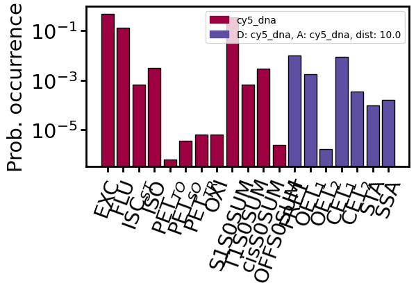
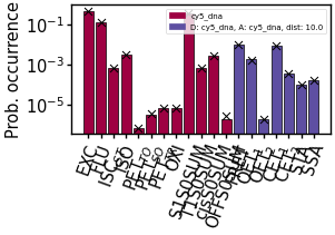
prediction.plot_frequency_transitions(scale=1)
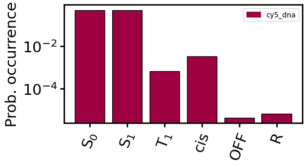
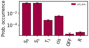
prediction.plot_frequency_states(scale=1)

array([[<Axes: ylabel='Prob. occurrence'>]], dtype=object)

Run a simulation

simulation = si.Simulation(transition_set)
simulation

<fluopy.simulation.Simulation at 0x7008ccd912b0>

%%time
# simulate until it reaches given end_time
simulation.run(start_at=None, size=1e6, end_time=500, seed=rng, use_memmap=None)
mi.print_class(simulation)

Floating point precision error warning:
 The smallest safe increment is 5.68e-14.
 Everything drawn below this number might be rounded to zero
 when approaching the time limit of this simulation.
 Using the highest possible rate which occurs for example in state combination [1, 1]
 gives a probability of 7.75e-05 for a smaller increment to be drawn.

Attributes of <fluopy.simulation.Simulation object at 0x7008ccd912b0>:
.................................................................
transition_set = <fluopy.transitions.TransitionSet object at 0x7009103def90>
_________________________________________________________________
time_series = array([0.00000000e+00, 5.75837004e-08, 6.0586144...81150266e+02, 5.00000000e+02], shape=(22687295,))
_________________________________________________________________
transition_series = array([  0,  96,   1, ..., 106,  10,  70], shape=(22687293,), dtype=uint32)
_________________________________________________________________
state_series = array([[0, 0, 0, ..., 7, 7, 7],
       [0, 1, 0, ..., 0, 1, 7]], shape=(2, 22687294), dtype=int8)
_________________________________________________________________
memmap_path = None
_________________________________________________________________


CPU times: user 1min 6s, sys: 157 ms, total: 1min 6s
Wall time: 1min 6s

Analyze the simulation

analysis = an.Analysis(simulation=simulation)
mi.print_class(analysis)

Attributes of <fluopy.analysis.Analysis object at 0x7008ccd91400>:
.................................................................
simulation = <fluopy.simulation.Simulation object at 0x7008ccd912b0>
_________________________________________________________________
frequency_transitions = array([4.93169767e-01, 1.29110335e-01, 6.7883815... 3.59099695e-04, 1.00144164e-04, 1.63792128e-04])
_________________________________________________________________
frequency_states = {'cy5_dna': array([4.98053379e-01, 4.98053379e-01, 6.7181880...3435e-03,
       3.44611944e-06, 6.54326476e-06])}
_________________________________________________________________
transition_time_distributions = [array([1.60771192e-07, 5.14620749e-08, 2.7001028...86329713e-08, 9.42114298e-08], shape=(11188687,)), array([2.46836785e-09, 5.99342571e-12, 1.9523953....70265604e-10, 3.42532758e-09], shape=(2929164,)), array([3.32554442e-09, 1.21016084e-09, 1.7050239... 3.57761110e-09, 1.22037136e-09], shape=(15401,)), array([2.00663296e-09, 3.07114014e-10, 9.0759629... 2.08842721e-10, 1.45507784e-09], shape=(73620,)), array([1.76919881e-06, 8.02568351e-07, 1.1900283... 2.70325421e-06, 3.45086215e-06, 6.86523890e-07]), array([9.53683447e-10, 1.21147536e-12, 4.4465124... 4.28940439e-10, 4.95276709e-10, 1.00789066e-09]), ...]
_________________________________________________________________
lifetime_distributions = {'cy5_dna': [array([1.60771192e-07, 5.14620749e-08, 2.7001028...86329713e-08, 9.42114298e-08], shape=(11417543,)), array([2.93141396e-10, 4.38715019e-10, 2.4683678...77180937e-10, 1.00789066e-09], shape=(11417543,)), array([9.28066744e-07, 5.20142133e-07, 2.7614122... 4.88162186e-08, 3.24744178e-08], shape=(15401,)), array([9.28299589e-07, 1.33557993e-05, 5.6726824... 5.51811695e-07, 1.05429953e-05], shape=(73620,)), array([2.48218820e-02, 2.94804611e+01, 5.3698889...8137e-02, 3.59128428e+01,
       1.97457573e+01]), array([7.42170840e-04, 5.72825337e-04, 1.4633080...6747e-03,
       1.40326991e-03, 4.16235275e-04])]}
_________________________________________________________________
mean_transition_times = array([1.68868320e-07, 1.61985166e-09, 1.6100627... 1.46648458e-09, 1.62599836e-09, 1.50990176e-09])
_________________________________________________________________
mean_lifetimes = {'cy5_dna': array([1.68461594e-07, 1.61689203e-09, 2.2119280...4157e-05,
       1.23085768e+01, 7.95602338e-04])}
_________________________________________________________________
state_occupations = {'cy5_dna': array([1.97075215e-03, 1.89152516e-05, 3.4904254...0361e-03,
       9.96307447e-01, 1.22277276e-04])}
_________________________________________________________________

analysis.get_fluorescence_lifetimes(fluorophore="cy5_dna")
analysis.get_emitting_transition_lifetimes(fluorophore="cy5_dna")

analysis.plot_frequency_transitions(scale=0.5, prediction=prediction)
analysis.plot_frequency_states(scale=0.5, prediction=prediction)
# analysis.plot_mean_transition_times(scale=0.5, prediction=prediction)
# analysis.plot_mean_lifetimes(scale=0.5, prediction=prediction)
# analysis.plot_state_occupations(scale=0.5, prediction=prediction)
# analysis.plot_lifetime_distributions(
#    scale=0.5, prediction=prediction, fluorophore="cy5_dna", state_identity=1
# )
# analysis.plot_transition_time_distributions(
#    scale=0.5, prediction=prediction, fluorophore="cy5_dna", transition_id=0
# )

array([[<Axes: ylabel='Prob. occurrence'>]], dtype=object)

Simulation of experimentally observable (photons per frames) only

Extract photon emission events from simulation

%%time
emissions = em.Emissions(frame_time="5ms", seed=rng, bandpass=(600, 800))
emissions.extract(simulation=simulation)
emissions

CPU times: user 978 ms, sys: 4 ms, total: 982 ms
Wall time: 981 ms

<fluopy.emissions.Emissions at 0x7008cca2da90>

Simulate photon emission events

Correct for detection efficiency and noise contributions:

emissions.add_photon_collection_objective(p=0.1, seed=rng)  # 1.
emissions.add_quantum_efficiency(p=0.9, seed=rng)  # 3.1.
emissions.add_poisson_noise(
    rate=0.05, seed=rng
)  # 3.2. (dark noise), note the frame time
emissions.add_emccd_gain(emccd_gain=10, seed=rng)  # 4.
emissions.add_gaussian_noise(mean=10, std=1, seed=rng)  # 5. (readout noise)
emissions

<fluopy.emissions.Emissions at 0x7008cca2da90>

emissions = em.Emissions(frame_time=”5ms”, seed=rng, bandpass=(660, 700)) emissions.extract(simulation=approximation)

# 2.
# at this point, the bandpass filter was applied
# yet, the effect of photon collection by the objective is missing
# the order is not relevant for two consecutive binomial distributions
# it is more convenient to apply the bandpass first because it needs the
# information about the emitting fluorophore whereas all the other effects are
# roughly wavelength independent
p_photon_collection = fo.calculate_photon_collection_rate(NA=1.45, n1=1.51)
emissions.add_photon_collection_objective(p=p_photon_collection)  # 1.
emissions.add_quantum_efficiency(p=0.9)  # 4.1.
emissions.add_transmittance(p=0.99)  # 3 (depending on number of components of optical
# path, may be applied multiple times)
emissions.add_poisson_noise(rate=0.05)  # 4.2. (dark noise), note the frame time
emissions.add_emccd_gain(emccd_gain=10)  # 5. (+ multiplicative noise)
emissions.add_gaussian_noise(mean=10, std=1, seed=rng)  # 6. (readout noise)
# CIC (spurious noise) neglected since low probability to happen in the pixels of
# interest
emissions.apply_threshold(threshold=100)  # 7 (thresholding)

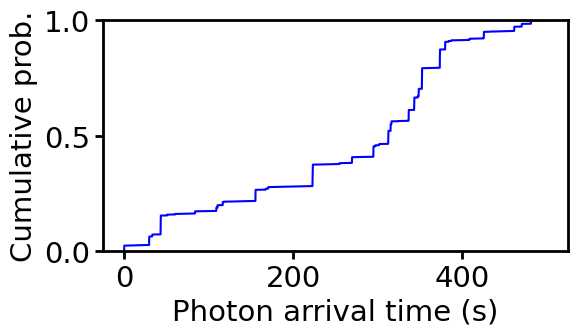
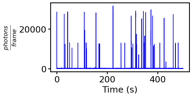
emissions.plot_cumulative_events(scale=1)
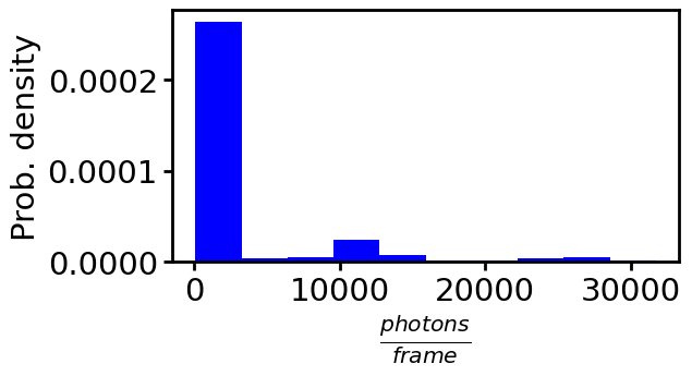
emissions.plot_histogram(scale=1)
emissions.plot_time_series(scale=1)

# to save the time_series and time_points
# emissions.save(path='', name_extension='test')

# to load time_series and time_points
# emissions.load(path='', name_extension='test')

array([[<Axes: xlabel='Time (s)', ylabel='$\\frac{photons}{frame}$'>]],
      dtype=object)

Simulation of pulsed excitation

%%time
emissions_tcspc = em.Emissions(frame_time="1ms", seed=rng, bandpass=None)
lifetimes_DA, lifetimes_D, lifetimes_all, simulation_object = emissions_tcspc.tcspc(
    transition_set=transition_set,
    number_pulses=5e5,
    pulse_duration=1e-11,
    time_between_pulses=1e-7,
    excitation_rates={"cy5_dna": 1e11},
    size=1e5,
    store_time_points=True,
    # details = True
)

the last frame (of index 0.05) has 1.00e+00 times the pulses of other frames.

CPU times: user 54.4 s, sys: 218 ms, total: 54.6 s
Wall time: 54.4 s

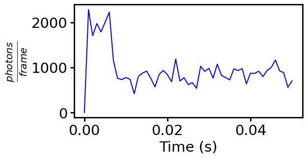
emissions_tcspc.plot_time_series()

array([[<Axes: xlabel='Time (s)', ylabel='$\\frac{photons}{frame}$'>]],
      dtype=object)

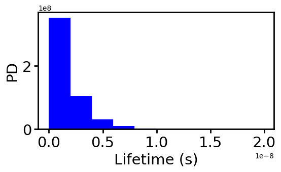
fi.universal_figure(
    type_="hist", data=lifetimes_all, ylabel="PD", density=True, xlabel="Lifetime (s)"
)

array([[<Axes: xlabel='Lifetime (s)', ylabel='PD'>]], dtype=object)

Fluorescence correlation spectroscopy

Observed fluorescence emission events can be analyzed by a correlation analysis.

fcs = fcs_p.FCS(emissions)
list(vars(fcs).keys())

['emissions', 'autocorrelation', 'tau']

Autocorrelation of time points

%%time
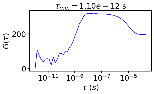
fcs.autocorrelate_time_points(
    exp_min=-20, exp_max=-6, points_per_base=4, base=4, normalize=True
)

CPU times: user 4.19 s, sys: 216 ms, total: 4.4 s
Wall time: 4.4 s

<fluopy.fcs.FCS at 0x7008cc366270>

mi.print_class(fcs)
fcs.plot(normalize_to=None, unit="s", scale=1);

Attributes of <fluopy.fcs.FCS object at 0x7008cc366270>:
.................................................................
emissions = <fluopy.emissions.Emissions object at 0x7008cca2da90>
_________________________________________________________________
autocorrelation = array([  0.        , 105.25773385,  74.42845738,...37465, 195.96795256, 195.71451995, 194.70409197])
_________________________________________________________________
tau = array([1.09785722e-12, 1.55260457e-12, 2.1957144... 1.04193529e-04, 1.47351902e-04, 2.08387058e-04])
_________________________________________________________________

Autocorrelation of time series

fcs.autocorrelate_time_series(log=True, m=4, normalize=True)

<fluopy.fcs.FCS at 0x7008cc366270>

fcs.plot(normalize_to=None, unit="s", scale=1);

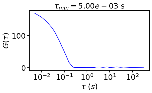
# some fcs fits are available:
# fcs_predict = fcs_p.fit_dark(tau, dark_lifetime, dark_occupation)
# fcs_predict = fcs_p.fit_antibunching(tau, excitation_rate, s1_lifetime)
# fcs_predict = fcs_p.fit_triplet_cis(tau, k_isc, k_T, k_01, k_10, k_iso, k_biso_eff)

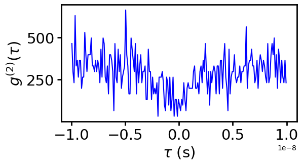
Antibunching

Alternatively, you can focus on fast time scales in a linear scale and observe antibunching.

# sensible to tau_max and bin_width, see coincidence notebook
hist, bins = fcs_p.coincidence(
    emissions.event_time_points[: int(2e5)], tau_max=1e-8, bin_width=1e-10, seed=rng
)
fi.universal_figure(
    type_="line",
    data=[bins, hist],
    xlabel=r"$\tau$ (s)",
    ylabel=r"$g^{(2)}(\tau)$",
    scale=1,
);

Blinking

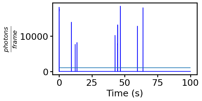
Emissions from a short simulation

We limit the dataset to 2000 frames for illustration purposes.

%%time
emissions = em.Emissions(frame_time="10ms", seed=rng, bandpass=None)
emissions.simulate(
    transition_set=transition_set, store_time_points=False, frames=10_000
)
emissions

CPU times: user 9.84 s, sys: 6.97 ms, total: 9.85 s
Wall time: 9.85 s

<fluopy.emissions.Emissions at 0x7008cca61bd0>

threshold: int = 1000

emissions.plot_time_series(scale=1)
plt.hlines(threshold, xmin=0, xmax=100)

<matplotlib.collections.LineCollection at 0x7008cc946a50>

blinks = bl.Blinking(emissions, threshold=threshold)
blinks

<fluopy.blinking.Blinking at 0x7008cca2fcb0>

mi.print_class(blinks)

Attributes of <fluopy.blinking.Blinking object at 0x7008cca2fcb0>:
.................................................................
emissions = <fluopy.emissions.Emissions object at 0x7008cca61bd0>
_________________________________________________________________
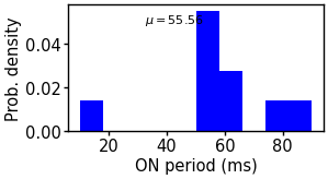
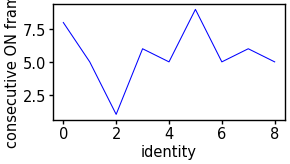
on_periods = array([8, 5, 1, 6, 5, 9, 5, 6, 5])
_________________________________________________________________
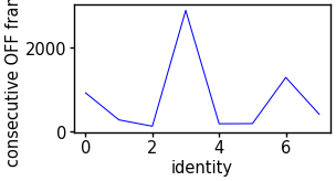
off_periods = array([ 927,  285,  134, 2889,  193,  197, 1294,  419])
_________________________________________________________________
on_periods_frames = array([   1,  936, 1226, 1361, 4256, 4454, 4660, 5959, 6384])
_________________________________________________________________
off_periods_frames = array([   9,  941, 1227, 1367, 4261, 4463, 4665, 5965])
_________________________________________________________________

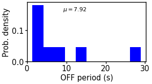
# plot a histogram of OFF times
blinks.plot(
    mode="off_histogram", density=True, display_mean=True, as_time="s", scale=0.5
)

# plot a histogram of ON times
blinks.plot(
    mode="on_histogram", density=True, display_mean=True, as_time="ms", scale=0.5
)

# plot a time series of OFF times
blinks.plot(mode="off_frame_series", scale=0.5)

# plot a time series of ON times
blinks.plot(mode="on_frame_series", scale=0.5)

array([[<Axes: xlabel='identity', ylabel='consecutive ON frames'>]],
      dtype=object)

# to get information of the photophysical (not analytical) OFF of each fluorophore, use
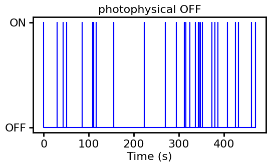
on_off_times_photophys, on_off_values_photophys = bl.get_off_statistics(
    simulation=simulation, index=0
)

# to get the analytical OFF statistics as the same view, use
on_off_times_analytic, on_off_values_analytic = bl.get_analytical_off_statistics(
    off_frames=blinks.off_periods_frames,
    off_periods=blinks.off_periods,
    on_frames=blinks.on_periods_frames,
    frame_time=blinks.emissions.parameters["frame_time"],
)

# plot the photophysical OFF statistics
bl.plot_off_statistics(
    on_off_times_photophys,
    on_off_values_photophys,
    scale=1,
    title="photophysical OFF",
)
# plot the analytical OFF statistics (no differentiation between fluorophores)
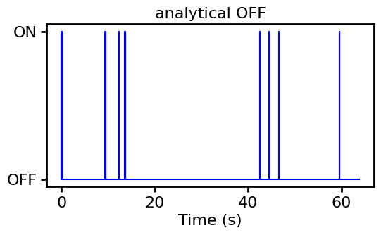
bl.plot_off_statistics(
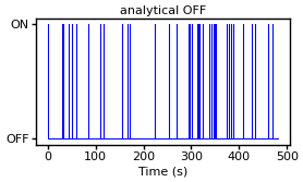
    on_off_times_analytic, on_off_values_analytic, scale=1, title="analytical OFF"
)

array([[<Axes: title={'center': 'analytical OFF'}, xlabel='Time (s)'>]],
      dtype=object)

Emissions from the long simulation

Get more detailed information from a complete simulation:

%%time
emissions = em.Emissions(frame_time="10ms", seed=rng, bandpass=None)
emissions.extract(simulation=simulation)
emissions

CPU times: user 963 ms, sys: 8.98 ms, total: 972 ms
Wall time: 972 ms

<fluopy.emissions.Emissions at 0x7008cc846060>

blinks = bl.Blinking(emissions, threshold=threshold)
blinks

<fluopy.blinking.Blinking at 0x7008be43f9d0>

mi.print_class(blinks)

Attributes of <fluopy.blinking.Blinking object at 0x7008be43f9d0>:
.................................................................
emissions = <fluopy.emissions.Emissions object at 0x7008cc846060>
_________________________________________________________________
on_periods = array([ 6, 12,  4, 22,  2,  1,  4,  5,  4,  7,  ..., 21,  9,  2,  2,  3,
       10,  1,  7,  6,  6])
_________________________________________________________________
off_periods = array([2945,  351,  991,  755,  948, 2349, 2504,... 293, 2152,
       1705,  713, 2872,  881, 1087])
_________________________________________________________________
on_periods_frames = array([    1,  2952,  3315,  4310,  5087,  6037,...40825, 42533, 43256,
       46129, 47017, 48110])
_________________________________________________________________
off_periods_frames = array([    7,  2964,  3319,  4332,  5089,  6038,...38673, 40828, 42543, 43257,
       46136, 47023])
_________________________________________________________________

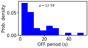
# plot a histogram of OFF times
blinks.plot(
    mode="off_histogram", density=True, display_mean=True, as_time="s", scale=0.5
)

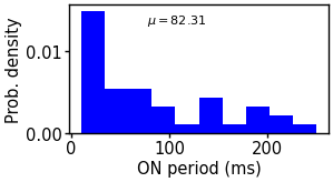
# plot a histogram of ON times
blinks.plot(
    mode="on_histogram", density=True, display_mean=True, as_time="ms", scale=0.5
)

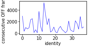
# plot a time series of OFF times
blinks.plot(mode="off_frame_series", scale=0.5)

# plot a time series of ON times
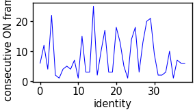
blinks.plot(mode="on_frame_series", scale=0.5)

array([[<Axes: xlabel='identity', ylabel='consecutive ON frames'>]],
      dtype=object)

# to get information of the photophysical (not analytical) OFF of each fluorophore, use
on_off_times_photophys, on_off_values_photophys = bl.get_off_statistics(
    simulation=simulation, index=0
)

# to get the analytical OFF statistics as the same view, use
on_off_times_analytic, on_off_values_analytic = bl.get_analytical_off_statistics(
    off_frames=blinks.off_periods_frames,
    off_periods=blinks.off_periods,
    on_frames=blinks.on_periods_frames,
    frame_time=blinks.emissions.parameters["frame_time"],
)

# plot the photophysical OFF statistics
bl.plot_off_statistics(
    on_off_times_photophys,
    on_off_values_photophys,
    scale=1,
    title="photophysical OFF",
)
# plot the analytical OFF statistics (no differentiation between fluorophores)
bl.plot_off_statistics(
    on_off_times_analytic, on_off_values_analytic, scale=0.5, title="analytical OFF"
)

array([[<Axes: title={'center': 'analytical OFF'}, xlabel='Time (s)'>]],
      dtype=object)