Tutorial about fluopy - Cy5 simulation

Here we outline a simulation procedure for typcial Cy5 fluorophore.

from pprint import pprint

%matplotlib inline

import numpy as np

import fluopy
import fluopy.analysis as an
import fluopy.emissions as em
import fluopy.fcs as fcs_p
import fluopy.figure as fi
import fluopy.fluorophores as fl
import fluopy.formulas as fo
import fluopy.miscellaneous as mi
import fluopy.prediction as pr
import fluopy.simulation as si
import fluopy.transitions as tr

fluopy.__version__

'0.4.0.dev4+gc3c2cb30d'

rng = np.random.default_rng(seed=1)

Define the fluorophore system

fluorophore = fl.Fluorophore(name="cy5_dna", position=[0, 0])
fluorophore_system = fl.FluorophoreSystem(fluorophores=[fluorophore])

pprint(vars(fluorophore_system))

{'count': 1,
 'distances': {},
 'fluorophores': [Fluorophore(identity=0,
                              name='cy5_dna',
                              position=array([0, 0]),
                              constants=FluorophoreData(data_files='cy5_data',
                                                        QUANTUM_YIELD=0.27,
                                                        FLUORESCENCE_LIFETIME=1.7e-09,
                                                        S1_QUENCH_RATE=0,
                                                        ISC_ST_RATE=830000.0,
                                                        ISC_TS_RATE=5000.0,
                                                        RISC_RATE=0,
                                                        STA_EFFICIENCY=0,
                                                        PHOTOBLEACH_T1_RATE=10.0,
                                                        PHOTOBLEACH_T2_RATE=0,
                                                        DSTORM_PET_T_RATE_MOL=100000000.0,
                                                        DSTORM_PET_S_RATE_MOL=1000000000.0,
                                                        DSTORM_PET_SUCCESS_RATE=0.001,
                                                        DSTORM_TH_EL_RATE_1=0.01,
                                                        DSTORM_TH_EL_RATE_2=0,
                                                        DSTORM_P_EL_CROSS_SECTION=6e-24,
                                                        RAD_ESCAPE_EFFICIENCY=0.01,
                                                        RAD_RELAX_RATE=1300.0,
                                                        OFRET_EFFICIENCY=0.001,
                                                        ISO_RATE=4000000.0,
                                                        BISO_CROSS_SECTION=6e-18,
                                                        BISO_THERMAL_RATE=5000.0,
                                                        BISO_EFFICIENCY=0.04,
                                                        H2O_ATTACK_S=0,
                                                        H2O_ATTACK_T=0,
                                                        BACK_REACTION=0))],
 'multi_type': False}

Define the transition set

transitions = fluorophore_system.load_transitions(
    summarize=True,
    irradiance=2,
    wavelength=640,
    bleaching=False,
    energy_transfer=False,
    dstorm=False,
)
transition_set = tr.TransitionSet(transitions, fluorophore_system)
transition_set = transition_set.remove_energy_transfers()
transition_set.finalize()

<fluopy.transitions.TransitionSet at 0x7c8fa6472c10>

transition_set.plot(graph_type="shell", colors=None, scale=1);

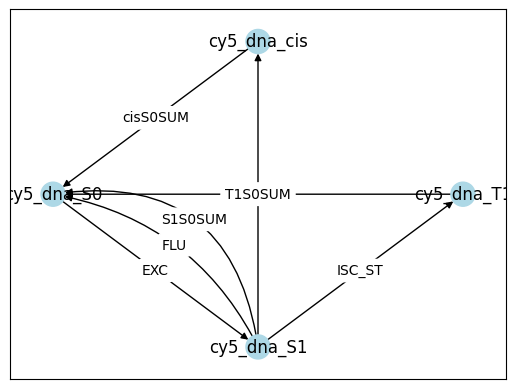
transition_set.transition_df

		transition_type	abbreviation	initial_state	final_state	rate	photon	fluorophore_ids	absorbing
Fluorophore	identity
cy5_dna	0	TransitionType.EXCITATION	EXC	SingleState.S0	SingleState.S1	5.815700e+06	False	[0]	False
	1	TransitionType.FLUORESCENT_EMISSION	FLU	SingleState.S1	SingleState.S0	1.588235e+08	True	[0]	False
	2	TransitionType.INTERSYSTEM_CROSSING_ST	ISC_ST	SingleState.S1	SingleState.T1	8.300000e+05	False	[0]	False
	3	TransitionType.ISOMERIZATION	ISO	SingleState.S1	SingleState.cis	4.000000e+06	False	[0]	False
	4	TransitionType.S1_S0_TRANSITIONS	S1S0SUM	SingleState.S1	SingleState.S0	4.245818e+08	False	[0]	False
	5	TransitionType.T1_S0_TRANSITIONS	T1S0SUM	SingleState.T1	SingleState.S0	5.000000e+03	False	[0]	False
	6	TransitionType.CIS_S0_TRANSITIONS	cisS0SUM	SingleState.cis	SingleState.S0	4.366202e+04	False	[0]	False

Make a prediction

%%time
prediction = pr.Prediction(transition_set)
prediction

CPU times: user 7.1 ms, sys: 18 μs, total: 7.12 ms
Wall time: 6.95 ms

<fluopy.prediction.Prediction at 0x7c8fa6372120>

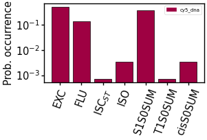
prediction.plot_frequency_transitions(scale=0.5)
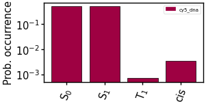
prediction.plot_frequency_states(scale=0.5)
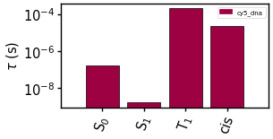
prediction.plot_mean_lifetimes(scale=0.5)
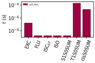
prediction.plot_mean_transition_times(scale=0.5)
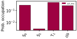
prediction.plot_state_occupations(scale=0.5)
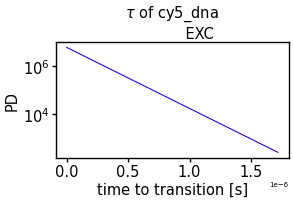
prediction.plot_transition_time_distributions(
    fluorophore="cy5_dna", transition_id=0, scale=0.5
);

Run a simulation

simulation = si.Simulation(transition_set)
simulation

<fluopy.simulation.Simulation at 0x7c8fa6333cb0>

%%time
# simulate until it reaches given end_time
simulation.run(start_at=None, size=1e6, end_time=2, seed=rng, use_memmap=None)
mi.print_class(simulation)

Floating point precision error warning:
 The smallest safe increment is 4.44e-16.
 Everything drawn below this number might be rounded to zero
 when approaching the time limit of this simulation.
 Using the highest possible rate which occurs for example in state combination [1]
 gives a probability of 2.61e-07 for a smaller increment to be drawn.

Attributes of <fluopy.simulation.Simulation object at 0x7c8fa6333cb0>:
.................................................................
transition_set = <fluopy.transitions.TransitionSet object at 0x7c8fa6472c10>
_________________________________________________________________
time_series = array([0.00000000e+00, 1.15167401e-07, 1.1846001....00000000e+00, 2.00000000e+00], shape=(6524933,))
_________________________________________________________________
transition_series = array([0, 4, 0, ..., 0, 4, 0], shape=(6524931,), dtype=uint32)
_________________________________________________________________
state_series = array([[0, 1, 0, ..., 1, 0, 1]], shape=(1, 6524932), dtype=int8)
_________________________________________________________________
memmap_path = None
_________________________________________________________________


CPU times: user 19.4 s, sys: 65 ms, total: 19.5 s
Wall time: 19.5 s

Analyze the simulation

analysis = an.Analysis(simulation=simulation)
mi.print_class(analysis)

Attributes of <fluopy.analysis.Analysis object at 0x7c8fa6332510>:
.................................................................
simulation = <fluopy.simulation.Simulation object at 0x7c8fa6333cb0>
_________________________________________________________________
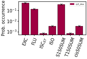
frequency_transitions = array([0.49794994, 0.13444157, 0.00071924, 0.00338103, 0.35940794,
       0.00071924, 0.00338103])
_________________________________________________________________
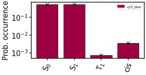
frequency_states = {'cy5_dna': array([0.49794986, 0.49794986, 0.00071924, 0.00338103])}
_________________________________________________________________
transition_time_distributions = [array([1.15167401e-07, 2.00370096e-07, 1.0292415....63219744e-07, 1.45854854e-07], shape=(3249089,)), array([2.70692572e-09, 1.04365849e-09, 1.1245765...3.31317862e-10, 4.92114571e-10], shape=(877222,)), array([8.13131906e-11, 1.12316807e-09, 3.2367626..., 5.40452016e-09, 2.11550555e-09], shape=(4693,)), array([2.78520369e-11, 4.96192071e-11, 5.2462151... 2.00435224e-11, 1.59720193e-09], shape=(22061,)), array([3.29261809e-09, 3.21472338e-10, 4.8111506....61337743e-09, 1.19445209e-09], shape=(2345112,)), array([2.09049325e-04, 4.70720765e-05, 3.1177581..., 1.86038850e-04, 4.51610664e-04], shape=(4693,)), ...]
_________________________________________________________________
lifetime_distributions = {'cy5_dna': [array([1.15167401e-07, 2.00370096e-07, 1.0292415....63219744e-07, 1.45854854e-07], shape=(3249089,)), array([3.29261809e-09, 3.21472338e-10, 4.8111506....61337743e-09, 1.19445209e-09], shape=(3249088,)), array([2.09049325e-04, 4.70720765e-05, 3.1177581..., 1.86038850e-04, 4.51610664e-04], shape=(4693,)), array([2.30303056e-05, 1.90388195e-05, 9.5060310... 1.90693565e-05, 6.86694646e-06], shape=(22061,))]}
_________________________________________________________________
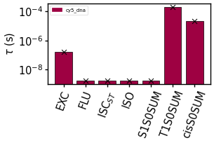
mean_transition_times = array([1.72109674e-07, 1.70175727e-09, 1.6878776... 1.70059714e-09, 1.98908089e-04, 2.27459440e-05])
_________________________________________________________________
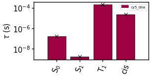
mean_lifetimes = {'cy5_dna': array([1.72109674e-07, 1.70091481e-09, 1.98908089e-04, 2.27459440e-05])}
_________________________________________________________________
state_occupations = {'cy5_dna': array([0.27959982, 0.00276321, 0.46673783, 0.25089914])}
_________________________________________________________________

analysis.get_fluorescence_lifetimes(fluorophore="cy5_dna")
analysis.get_emitting_transition_lifetimes(fluorophore="cy5_dna")

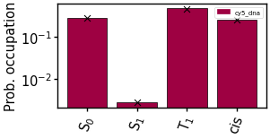
analysis.plot_frequency_transitions(scale=0.5, prediction=prediction)
analysis.plot_frequency_states(scale=0.5, prediction=prediction)
analysis.plot_mean_transition_times(scale=0.5, prediction=prediction)
analysis.plot_mean_lifetimes(scale=0.5, prediction=prediction)
analysis.plot_state_occupations(scale=0.5, prediction=prediction)
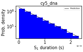
analysis.plot_lifetime_distributions(
    scale=0.5, prediction=prediction, fluorophore="cy5_dna", state_identity=1
)
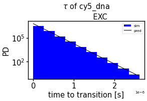
analysis.plot_transition_time_distributions(
    scale=0.5, prediction=prediction, fluorophore="cy5_dna", transition_id=0
)

array([[<Axes: title={'center': '$\\tau$ of cy5_dna\n            EXC'}, xlabel='time to transition [s]', ylabel='PD'>]],
      dtype=object)

Simulation of experimentally observable (photons per frames) only

Extract photon emission events from simulation

%%time
emissions = em.Emissions(frame_time="5ms", seed=rng, bandpass=(600, 800))
emissions.extract(simulation=simulation)
emissions

CPU times: user 289 ms, sys: 3 ms, total: 292 ms
Wall time: 292 ms

<fluopy.emissions.Emissions at 0x7c8fa6332ba0>

Simulate photon emission events

Correct for detection efficiency and noise contributions:

emissions.add_photon_collection_objective(p=0.1, seed=rng)  # 1.
emissions.add_quantum_efficiency(p=0.9, seed=rng)  # 3.1.
emissions.add_poisson_noise(
    rate=0.05, seed=rng
)  # 3.2. (dark noise), note the frame time
emissions.add_emccd_gain(emccd_gain=10, seed=rng)  # 4.
emissions.add_gaussian_noise(mean=10, std=1, seed=rng)  # 5. (readout noise)
emissions

<fluopy.emissions.Emissions at 0x7c8fa6332ba0>

emissions = em.Emissions(frame_time=”5ms”, seed=rng, bandpass=(660, 700)) emissions.extract(simulation=approximation)

# 2.
# at this point, the bandpass filter was applied
# yet, the effect of photon collection by the objective is missing
# the order is not relevant for two consecutive binomial distributions
# it is more convenient to apply the bandpass first because it needs the
# information about the emitting fluorophore whereas all the other effects are
# roughly wavelength independent
p_photon_collection = fo.calculate_photon_collection_rate(NA=1.45, n1=1.51)
emissions.add_photon_collection_objective(p=p_photon_collection)  # 1.
emissions.add_quantum_efficiency(p=0.9)  # 4.1.
emissions.add_transmittance(p=0.99)  # 3 (depending on number of components of optical
# path, may be applied multiple times)
emissions.add_poisson_noise(rate=0.05)  # 4.2. (dark noise), note the frame time
emissions.add_emccd_gain(emccd_gain=10)  # 5. (+ multiplicative noise)
emissions.add_gaussian_noise(mean=10, std=1, seed=rng)  # 6. (readout noise)
# CIC (spurious noise) neglected since low probability to happen in the pixels of
# interest
emissions.apply_threshold(threshold=100)  # 7 (thresholding)

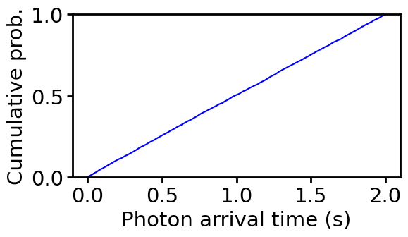
emissions.plot_cumulative_events(scale=1)
emissions.plot_histogram(scale=1)
emissions.plot_time_series(scale=1)

# to save the time_series and time_points
# emissions.save(path='', name_extension='test')

# to load time_series and time_points
# emissions.load(path='', name_extension='test')

array([[<Axes: xlabel='Time (s)', ylabel='$\\frac{photons}{frame}$'>]],
      dtype=object)

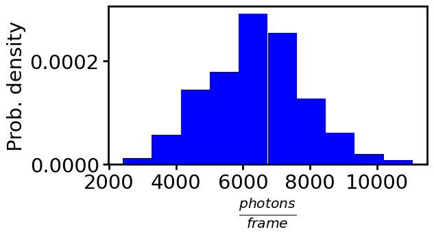
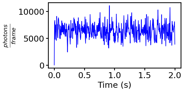
Simulation of pulsed excitation

%%time
emissions_tcspc = em.Emissions(frame_time="10us", seed=rng, bandpass=None)
lifetimes_DA, lifetimes_D, lifetimes_all, simulation_object = emissions_tcspc.tcspc(
    transition_set=transition_set,
    number_pulses=5e5,
    pulse_duration=1e-11,
    time_between_pulses=1e-7,
    excitation_rates={"cy5_dna": 1e11},
    size=1e5,
    store_time_points=True,
    # details = True
)

the last frame (of index 0.05) has 1.00e+00 times the pulses of other frames.

CPU times: user 27.8 s, sys: 433 ms, total: 28.2 s
Wall time: 27.7 s

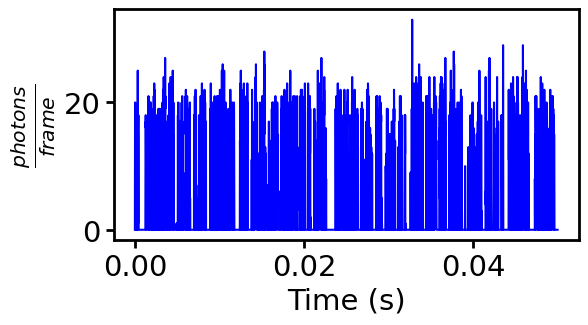
emissions_tcspc.plot_time_series()
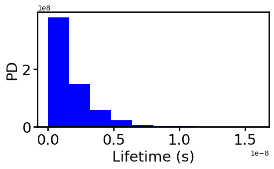
fi.universal_figure(
    type_="hist", data=lifetimes_all, ylabel="PD", density=True, xlabel="Lifetime (s)"
)

array([[<Axes: xlabel='Lifetime (s)', ylabel='PD'>]], dtype=object)

Fluorescence correlation spectroscopy

Observed fluorescence emission events can be analyzed by a correlation analysis.

fcs = fcs_p.FCS(emissions)
list(vars(fcs).keys())

['emissions', 'autocorrelation', 'tau']

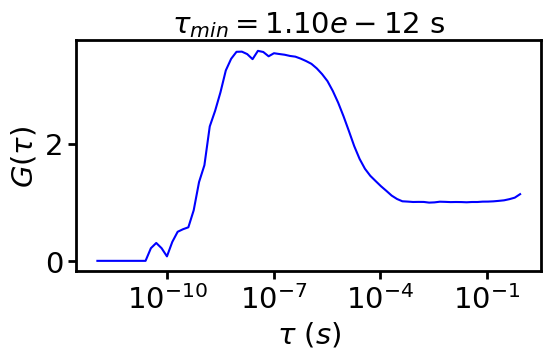
Autocorrelation of time points

%%time
fcs.autocorrelate_time_points(
    exp_min=-20, exp_max=0, points_per_base=4, base=4, normalize=True
)

CPU times: user 3.79 s, sys: 324 ms, total: 4.12 s
Wall time: 4.12 s

<fluopy.fcs.FCS at 0x7c8fa6332f90>

mi.print_class(fcs)
fcs.plot(normalize_to=None, unit="s", scale=1);

Attributes of <fluopy.fcs.FCS object at 0x7c8fa6332f90>:
.................................................................
emissions = <fluopy.emissions.Emissions object at 0x7c8fa6332ba0>
_________________________________________________________________
autocorrelation = array([0.        , 0.        , 0.        , 0.   ... 1.03173005, 1.05149662, 1.07705871, 1.13681592])
_________________________________________________________________
tau = array([1.09785722e-12, 1.55260457e-12, 2.1957144... 4.26776695e-01, 6.03553391e-01, 8.53553391e-01])
_________________________________________________________________

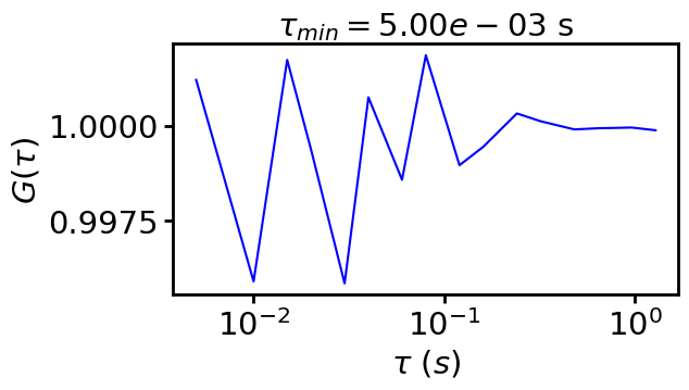
Autocorrelation of time series

fcs.autocorrelate_time_series(log=True, m=4, normalize=True)

<fluopy.fcs.FCS at 0x7c8fa6332f90>

fcs.plot(normalize_to=None, unit="s", scale=1);

# some fcs fits are available:
# fcs_predict = fcs_p.fit_dark(tau, dark_lifetime, dark_occupation)
# fcs_predict = fcs_p.fit_antibunching(tau, excitation_rate, s1_lifetime)
# fcs_predict = fcs_p.fit_triplet_cis(tau, k_isc, k_T, k_01, k_10, k_iso, k_biso_eff)

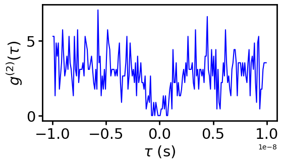
Antibunching

Alternatively, you can focus on fast time scales in a linear scale and observe antibunching.

# sensible to tau_max and bin_width, see coincidence notebook
hist, bins = fcs_p.coincidence(
    emissions.event_time_points[: int(2e5)], tau_max=1e-8, bin_width=1e-10, seed=rng
)
fi.universal_figure(
    type_="line",
    data=[bins, hist],
    xlabel=r"$\tau$ (s)",
    ylabel=r"$g^{(2)}(\tau)$",
    scale=1,
);